What is Lymann-\(\alpha\) Forest?
 Ly-\(\alpha\) forest example of QSO 1422+2309 (top panel), the interpretation of it’s formation (middle panel), and a zoom of the spectra (bottom panel). From Springel et al. (2006), Figure 2
When we look at the spectra of a quasar, we will find an area with very dense absorption lines blueward to the Lymann-\(\alpha\) emission line wavelength. This area looks like the forest, so it is called “Lymann-\(\alpha\) Forest”. Ly-\(\alpha\) forest, combined with two other kinds of absorption line (broad and narrow absorption line), raised a debate on their origin. It turned out that broad lines are from quasars themselves, while narrow lines as well as Ly-\(\alpha\) forest come from absorption of galaxies and neutral hydrogen located in the line-of-sight between quasar and us.
Photons with a wavelength of 1216 Angstrom may be absorbed by neutral hydrogen cloud in the line-of-sight between quasar and us. Although the absorption will always happen in 1216 Angstrom, the spectra of quasar, because of the expansion of Universe, will not stay in the same place. As the photon going through Universe, its wavelength will increase, that is, the whole spectra will have a redshift while the Lymann-\(\alpha\) absorption is still in the same wavelength. Thus, those dense absorption forest are mainly caused by one absorption (some other lines such as Lymann-\(\beta\) will also cause a “forest”, but much weaker than Lymann-\(\alpha\)).
A clear interpretation video is presented here.
Why Ly-\(\alpha\) Forest can be used as Cosmological Tool?
Because the absorption which should be in the same wavelength now shifted to a wavelength range corresponding to quasar’s redshift, it maps the situation of neutral hydrogen between the redshifted Lymann-\(\alpha\) line of quasar and 1216 Angstrom, and we can derive the distribution from what we have observed in the telescopes.
Furthermore, simulation and measurement of Lymann-\(\alpha\) line’s broadening indicate that density of neutral hydrogen cloud is low, and their temperature is between \(10^4\) and \(2 \times 10^4\). Compared to gravity, pressure forces will be small, so the behavior of neutral hydrogen will basically be the same as dark matter. As a result, we can trace density distribution also from that of neutral hydrogen.
Last but not least, the relation between observed flux in a particular wavelength and density in that distance can be determined, both from a complex relation or a easier method (Gallerani et al. 2011, see next section)
In short, the reason Ly-\(\alpha\) forest can be used as cosmological tool is by measuring it, we can constrain some parameters of our modeled cosmology, or, in reverse, we can create the model Ly-\(\alpha\) forest and it looks like what we actually observed.
How to constrain the model of Cosmology using Ly-\(\alpha\) Forest?
To constrain the cosmological parameters, we must first translate observed spectra to density fluctuation. It can be done by directly derive the relation from physical image, or using a more practical way. Gallerani et al. 2011 described both methods and it is worth repeating this here.
Since distribution of neutral hydrogen cloud is not homogenous along line-of-sight (LOS) between quasar and us, we have to treat each wavelength, or distance separately. We first divide the LOS into \(N\) bins, then as the definition of optical depth, we have,
\[\frac{F(i)}{F_c} = e^{-\tau(i)}\]where \(\tau(i)\) is,
\[\tau(i) = cI_\alpha \frac{\Delta x}{1+z(i)} \sum_{j=1}^{N} n_\mathrm{HI}(j)\Phi_\alpha[v_H(i) - v_H(j)]\]here \(c\) is light speed, \(I_\alpha\) represent the cross-section of hydrogen, \(\Delta x\) is the bin length in comoving coordinate, \(\Phi_\alpha\) is Voigt profile and \(n_\mathrm{HI}\) is neutral hydrogen fraction.
Neutral hydrogen cloud is in a low-density situation, so it’s easily ionized. We can assume that the cloud is in the equilibrium of ionization and recombination, then \(n_\mathrm{HI}\) can be express as:
\[n_\mathrm{HI} \propto \frac{T_0\Delta(j)^{-0.7(\gamma-1)}}{\Gamma} n_0^2 [1+z(j)]^3 \Delta(j)^2 \propto \Delta(j)^\beta, 1.5 < \beta < 2.0\]where \(T_0\) is IGM temperature at mean density and redshift \(z(j)\), \(\gamma\) (slope of equation of state) indicate the reionization history of Universe, \(\Gamma\) represent the photoionization rate at given \(z(j)\), and \(\Delta(j)\) is the over density in a given \(j\). So we can see here \(\tau(i)\) is related to the property of hydrogen cloud, reionization history of Universe and profile of hydrogen absorption line (even if assume Gaussian, it still related to thermal state of the gas).
This is the reason stating direct derivation of flux-density relation is very complex; it convolutes too many factors that makes calculation impossible or losing accuracy if more assumptions are introduced. However, by using probability distribution function (PDF), this relation can be determined by computation.
Let us now consider the PDF of observed, or transmitted flux \(F\) as well as over density \(\delta\). Here it is assumed that an over density \(\delta_*\) is associated to a single value of \(F_*\), so from the conservation of probability, integral from \(0\) to \(F_*\) must be equal to integration from \(\Delta_*\) to \(\infty\), that is,
\[\int_0^{F_*} P_F dF = \int_{\Delta_*}^\infty P_\Delta d\Delta\]or vice versa,
\[\int_{F_*}^1 P_F dF = \int_0^{\Delta_*} P_\Delta d\Delta\]Of course, observation will always be accompanied by uncertainties, so when the flux is very close to 0 or 1 we cannot tell the small discrepancy from 0 or 1 is from absorption or error. To account for this, one maximum and minimum flux (\(F_\mathrm{max}, F_\mathrm{min}\)) and the corresponding minimum and maximum optical depth (\(\Delta_\mathrm{min}, \Delta_\mathrm{max}\)) is set as the boundary of the integral,
\[\int_{F_\mathrm{min}}^{F_*} P_F dF = \int_{\Delta_*}^{\Delta_\mathrm{max}} P_\Delta d\Delta\] \[\int_{F_*}^{F_\mathrm{max}} P_F dF = \int_{\Delta_\mathrm{min}}^{\Delta_*} P_\Delta d\Delta\]By solving these equations, we can get the relation of \(F\) and \(\Delta\), then convert the observed spectra to over density. Simulation have shown that after setting a set of parameters \((\beta, \Gamma, T_0, \gamma)\), both the spectra and distribution of over density can be recover well.
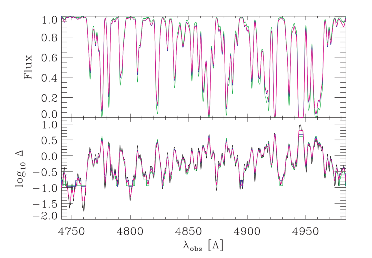 Top: Original spectra (black) of Ly-\(\alpha\) forest and synthetic spectra (red, blue and green) using different set of \((\Gamma, T_0, \gamma)\); bottom: same color for top but for distribution of overdensities. From Gallerani et al. 2011, Figure 3
So now we can determine a 1-dimentional density fluctuation long one LOS; this is far from enough to constrain the cosmological model. But if we have a large number of quasars spreading over a large area of celestial sphere, then it will be possible to achieve 3-D density field. Luckily, BOSS survey from SDSS provides this possibility.
 Footprint of BOSS; from Dawson et al. 2013
Recovering topology and power spectrum
Although with the data of BOSS survey, 3-D density distribution is possible to be derived, the separation of each quasar in slightly shifted LOS block us from directly detecting the distribution in between. As a result, interpolation have to be done.
Both Caucci ei al. 2008 and Kitaura et al. 2012 use a Bayesian method to interpolate. A detailed description is present in Pichon et al. 2001, and here only a summarize of this method will be present.
The relation between optical depth and neutral hydrogen is,
\[\tau_l(w) = \frac{c\sigma_0}{H(\bar{z})\sqrt{\pi}} \int \int \int_{-\infty}^{\infty} \frac{n_\mathrm{HI}(x,\mathbf{x}_\perp)}{b(x,\mathbf{x}_\perp)} \exp{\frac{[w-x-v_p(x,\mathbf{x}_\perp)]^2}{b(x,\mathbf{x}_\perp)^2}}dx \delta_D(\mathbf{x}_\perp,\mathbf{x}_{\perp,l})d^2 \mathbf{x}_{\perp,l}\]With some assumption of dark matter, we can translate \(n_\mathrm{HI}\) to density of dark matter \(\rho_\mathrm{DM}\). However, this relation still depends on many other parameters, so we have to determine them first.
Combining all those parameters, we can make an array, \(\mathbf{M}\), and what we want now is the probability of getting \(\mathbf{M}\) from a given data, \(\mathbf{D}\). According to Bayesian theorem, we have,
\[f(\mathbf{M} | \mathbf{D}) = \mathcal{L}(\mathbf{D} | \mathbf{M})f(\mathbf{M})\]which we can (though still a little complicated), compute the likelihood \(\mathcal{L}(\mathbf{D} \| \mathbf{M})\) and derive the prior \( f(\mathbf{M}) \) under some observation. Then, after holding the 3-D density result, visualization can be easily done.
Caucci ei al. 2008 recover the tropology of HI density field at redshift of 2 simulated by model. The result looks very consistent with the simulated data.
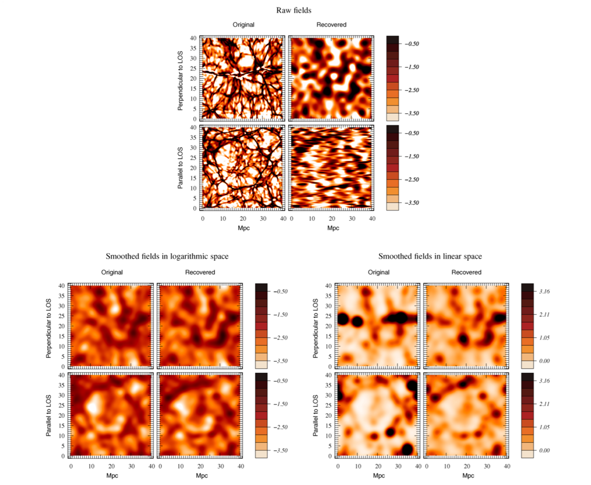 Comparison between original HI density field and recovered density field. Top row indicates the unsmoothed field, while bottom row is smoothed. From Caucci ei al. 2008, Figure 9
It is clear that the recovered density field is in a low resolution, because of the discrete distribution of LOS. But after smoothing at a scale larger than the LOS’s separation, we can hardly tell the difference of the original and recovered. Another point worth mentioning is that the recovery in logarithmic space is better than that in linear space.
Kitaura et al. 2012 recovered the power spectrum of density from simulation, and the result is again consist very well.
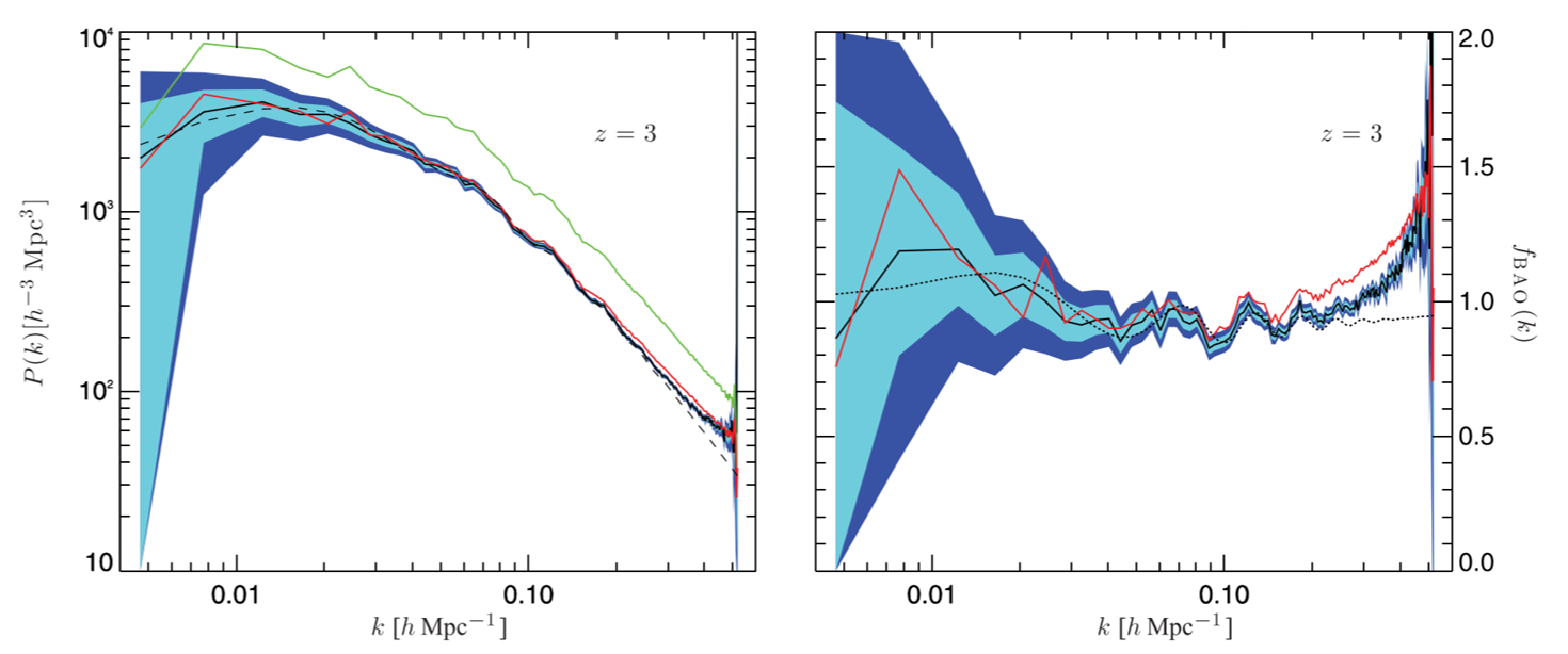 Comparison of simulated and recovered power spectrum. Red is from simulation, and black is recovered. From Kitaura et al. 2012, Figure 7
Measuring BAO feature from correlation function
A more straightforward constrain on cosmological model is from Busca et al. 2013. The spectra obtained by BOSS is still too sparse in the celestial sphere and the resolution is not high enough to directly recover the density distribution. This may be also the reason which Caucci ei al. 2008 and Kitaura et al. 2012 only provide the tool and use simulated data to recover. Instead correlation function of flux maybe more useful.
To achieve this, Busca et al. 2013 created correlation function as,
\[\hat{\xi}_A = \sum_{ij\in A}w_{ij}\delta_i\delta_j / \sum_{ij\in A} w_{ij}\]where
\[\delta(\lambda) = \frac{f(\lambda)}{C(\lambda)\bar{F}(z)} - 1\]\(w_{ij}\) is the weight of two corresponding pixel in two near quasars, \(f(\lambda)\) is observed flux, and \(C(\lambda)\bar{F}(z)\) is continuum. Volume \(A\) contains all quasars have a distance smaller than \(r\) to one quasar. So if the spectra of two quasars is similar, \(\hat{\xi}_A\) will be bigger than two whose spectra is not.
Now we can expect that in the sound horizon, the correlation function will have a (at least local) maximum, and the position of this peak will provide constrain on cosmological model.
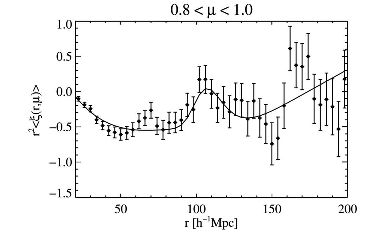 \(\xi(r,\mu)\) averaged over \(0.8 < \mu < 1\). From Busca et al. 2013, Figure 8
Indeed, the correlation function peaks at around 150 Mpc. \(\mu\) here correspond to the transvers direction of or along the LOS, where \(\mu\) near 1 means only selecting sources along LOS. Location of this peak can be used to constrain the real position of BAO peak through two multiplicative factors; and they are related to \(\Omega_m\) and \(\Omega_\Lambda\) separately, so constrain on multiplicative factors can be converted to constrains on cosmological parameters.
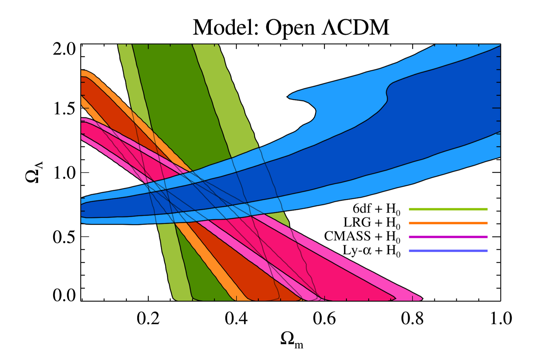 Constrains on matter and dark-energy density parameters determined by different method. From Busca et al. 2013, Figure 18
Combined with other constrains from different method, \(\Omega_m\) and \(\Omega_\Lambda\) of model \(\mathrm{\Lambda CDM}\) can be determined much better. Constrain by Ly-\(\alpha\) forest provide a distribution perpendicular to other methods, and it is the only method indicated \(\Omega_\Lambda\) should be greater than 0.5 (or, dark energy is needed).
Furthermore, after adding some constrains called WMAP7 that some parameters effecting multiplicative factors should change in the same direction, Hubble constant in redshift 2.3 \(H(z=2.3)\) can also be determined.
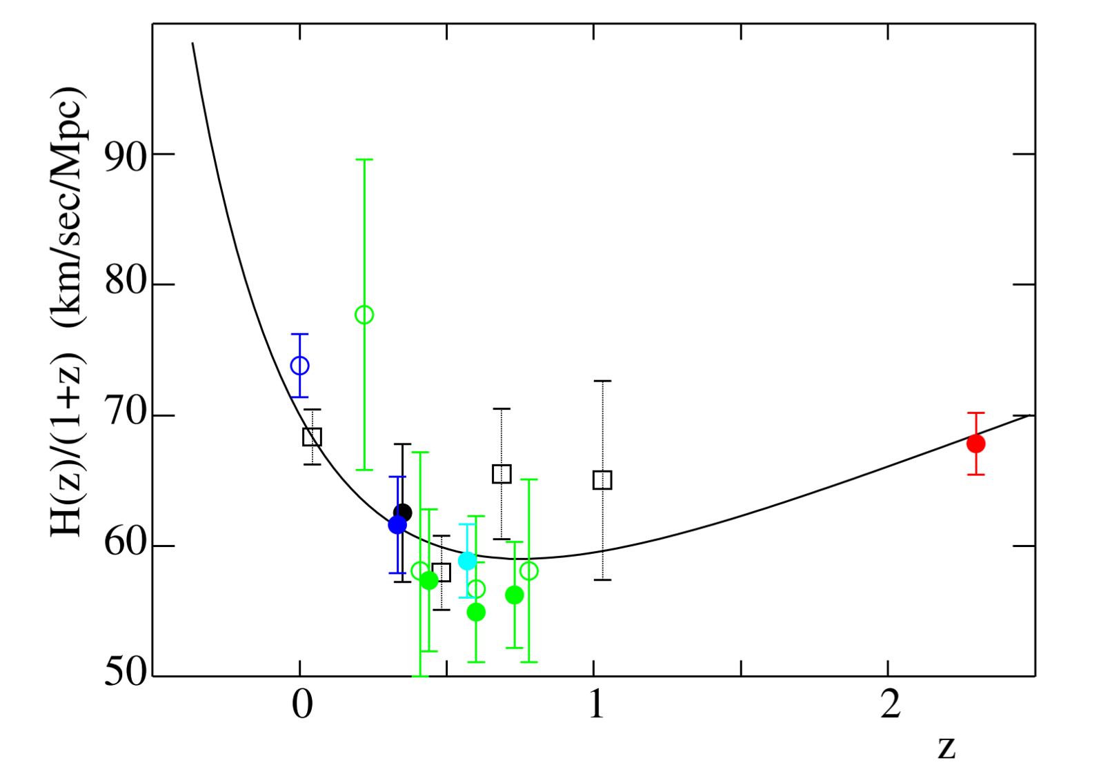 Measurements of \(H(z)/(1+z)\) vs \(z\); result of BAO measurement is the red dot. From Busca et al. 2013, Figure 21
This determination largely expand the redshift range. Without this datapoint, it is not clear that the \(H(z)\) in the past is flat or increasing or decreasing; now this measurement states that our Universe first experienced a decelerating expansion, then turn to accelerating expansion at redshift between 0 and 1.
Future
The future of Ly-\(\alpha\) forest is of course the future of quasar observation. Near future sees the successor of BOSS survey, eBOSS. More and deeper quasar will enhance the completeness of our measurement and help us to trace earlier epoch. Combining data from BOSS and eBOSS, we can have a better constrain on our model of Universe.
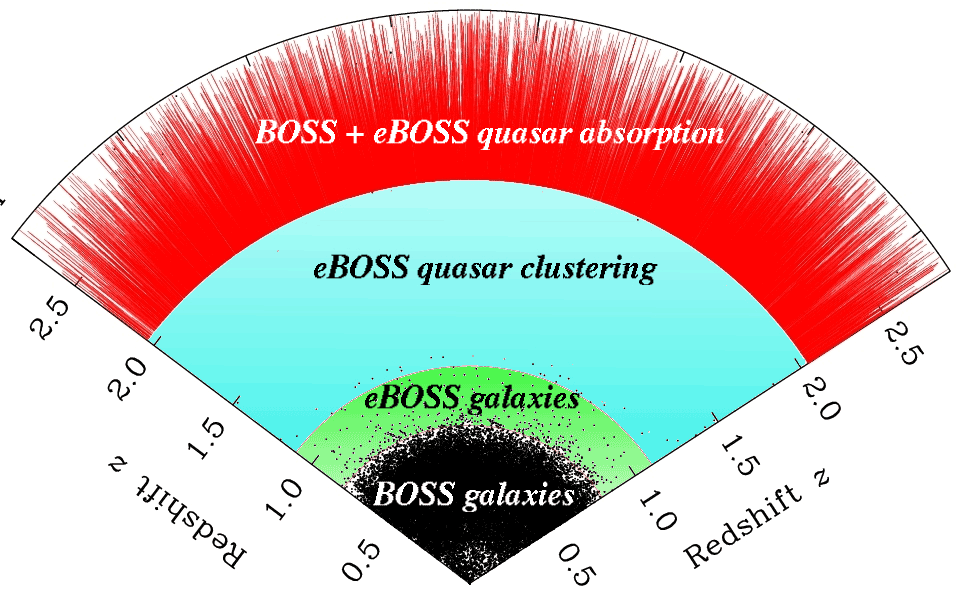 Planned eBOSS coverage of the Universe, from the webpage of eBOSS
References
- Schneider, P. Extragalactic Astronomy and Cosmology: An Introduction. (2015).
- Gallerani, S., Kitaura, F. S. & Ferrara, A. Cosmic density field reconstruction from Lyα forest data. Monthly Notices of the Royal Astronomical Society 413, L6–L10 (2011).
- Pichon, C., Vergely, J. L., Rollinde, E., Colombi, S. & Petitjean, P. Inversion of the Lyman α forest: three-dimensional investigation of the intergalactic medium. Monthly Notices of the Royal Astronomical Society 326, 597–620 (2001).
- Caucci, S. et al. Recovering the topology of the intergalactic medium at z ~ 2. Monthly Notices of the Royal Astronomical Society 386, 211–229 (2008).
- Kitaura, F. S., Gallerani, S. & Ferrara, A. Multiscale inference of matter fields and baryon acoustic oscillations from the Lyα forest. Monthly Notices of the Royal Astronomical Society 420, 61–74 (2012).
- Busca, N. G. et al. Baryon acoustic oscillations in the Lyα forest of BOSS quasars. Astronomy and Astrophysics 552, A96 (2013).